A Large Language Model Order Parameter
GPT-5 was released last week and marks another milestone in the rennaissance of modern AI. Despite quite a bit of vocal disappointment from some users, GPT-5 represents a major leap forward compared to the previous versions of OpenAI’s flagship Generative Pre-trained Transformer (GPT) model and steady progress in the rapidly evolving landscape of Large Language Models (LLMs) that can reason and use tools.
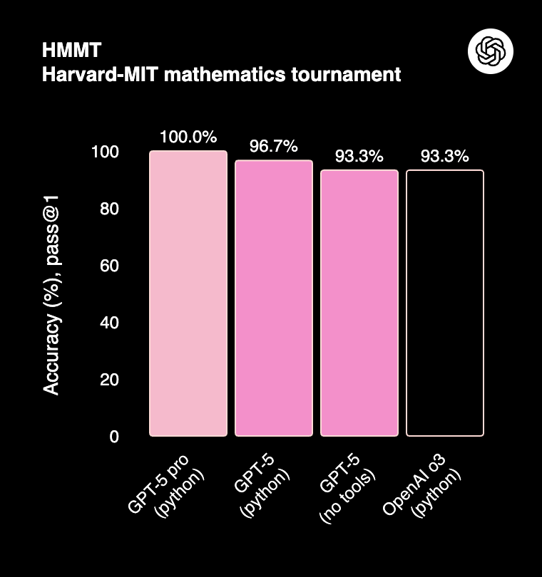
Figure 1: GPT-5 saturates the HMMT benchmark, a Harvard/MIT Mathematics Tournament for high school students. [Source]
Apart from acing high school math tests, multi-agent systems built using LLMs are now used for writing code, trading stocks, and seeking legal counsel. Their swift and widespread adoption in white collar jobs is a testament to the utility of AI models that can generate human language.
Building a GPT from scratch
The GPT model was introduced by OpenAI in 2018,1 building on the seminal paper called Attention is All You Need by Google researchers that first introduced the transformer architecture in 2017.2 In the original GPT paper, the language model was trained on
1) A diverse corpus of unlabeled text using unsupervised pre-training and
2) A set of labeled datasets encompassing text classification, sentence similarity, question answering, and natural language inference tasks using supervised finetuning.
In the current work, we follow Andrej Karpathy and focus on unsupervised pre-training of a language model on a small collection of Shakespeare’s plays. More specifically, we implement a slightly modified decoder-only transformer that uses multiple heads of masked self-attention and train it on character-level token and positional embeddings of the input text.
The goal of this training is to minimize the loss function to predict the next token (character) in the text:
Minimizing this \(\mathcal{L}(\theta)\) function by tuning the neural network parameters \(\theta\) allows the model to learn the rules of language to predict the next token accurately.
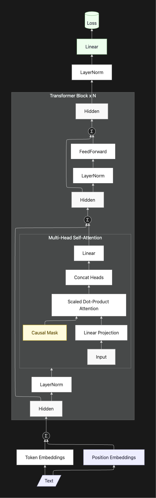
Figure 2: A Mermaid diagram of the Generative Pre-trained Transformer (GPT) model implemented here.
The end result is a language model that learns to regurgitate Shakespearean writing. For example, here’s a snippet of an output generated by this model:
ISABELLA: O, but special counsel your sorrows must be told. What counsel is but that? why can you breath?
JULIET: Know not wite, but what dost thou art? Bear then I’ll that ask it a forth of thee.
PARIS: How often have I have been my groan, And I will make you best your mistress of their business?
Well…maybe not, but its certainly better than anything I could come up with :)
Training Dynamics of Language Models
The Karpathy video that I followed to build this model finished training at 5000 steps but, interestingly (to me at least), training beyond this limit showed a curious observation:
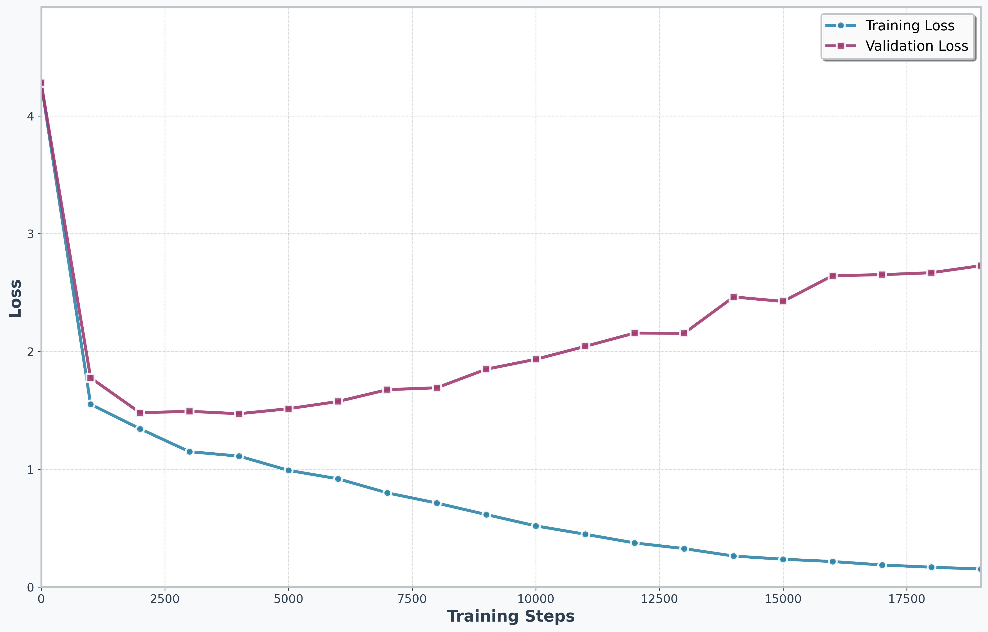
Figure 3: Loss as a function of training steps on Training and Valiation sets
Data processing for machine learning models typically involves splitting the available data into train/validation sets. This is done so that there is a held out set for validating the performance of the model beyond what it is already trained on. As in Figure 3, model performance on validation set degrades as one continues model training beyond a certain limit, as the model ends up “overfitting” on the training data.
The interesting part is that the “overfit” model does not perform poorly – in fact, the output shown above is actually generated after training completes 20,000 steps. This is because the loss function is designed to predict the next token and not, for example, predict labels in traditional supervised learning. This is one of the reasons why LLMs scale well.3
Through the Lenz of Statistical Physics
Another way to look at dynamics of neural network training could be through the lens of the Lenz-Ising Model or, as it is more commonly known as, the Ising Model.4 Ising Model is mainly a mathematical object that doesn’t correspond exactly to any physical system, but its properties have made it a popular tool for pedagogical statistical physics.
In a nutshell, Ising model refers to a lattice in d dimensions where each vertex \(s_i\) can have two identities: \(s_i = +1\) or \(s_i = -1\), i.e. spin up or down. These spins can be influenced by an external magnetic field \(h\) or via local interactions between neighboring vertices, with the interaction strength \(J_{i,j}\). Thus, the Hamiltonian of an Ising model can be written as:
This model has an analytical solution for the associated partition function in dimensions \(d=1\)5 and \(d=2\),6 but no-one has yet been able to solve it for the case \(d=3\). In higher dimensions, one typically uses the Mean Field Approximation to get to the solution. Crucially, the Ising model is popular because it exhibits disorder to order phase transitions in dimensions higher than 1, i.e. \(d>1\).7
The key connection to make is that the spins of the Ising model are analogous to the weights of the neural network underlying the LLM and, thus, one may define an order parameter that could give insight into the transition of an LLM from generating jumbled letters to something that looks like human language.
LLM Order Parameter
A recent paper8 has proposed an order parameter for arbitrary neural networks:
where \(\left\lVert W_{\text{head}}\right\rVert_F\) and \(d_{\text{model}}\) correspond to the norm and width of the final layer, in our case the LM Head (Linear) layer. We find that this order parameter increases monotonically with training duration and thus the loss function decreases monotonically with this order parameter. This observation is consistent across 4 orders of magnitude of the GPT model sizes - from 10,000 to 10,000,000 parameter models.
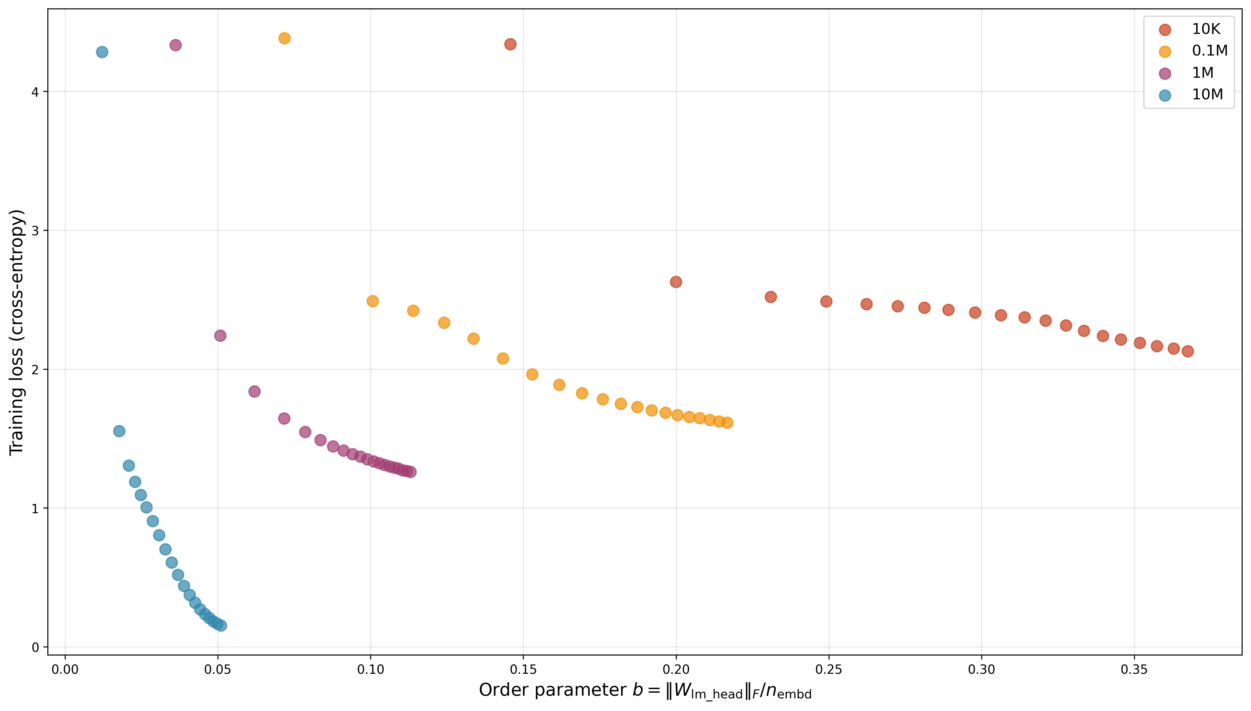
Figure 4: Training set loss as a function of the LLM Order Parameter for 4 different GPT model sizes, with number of parameters ranging from 10k to 10M.
A curious observation here is the change in the slope of graph observed in case of the two smaller models, though I’m not yet sure what it means…
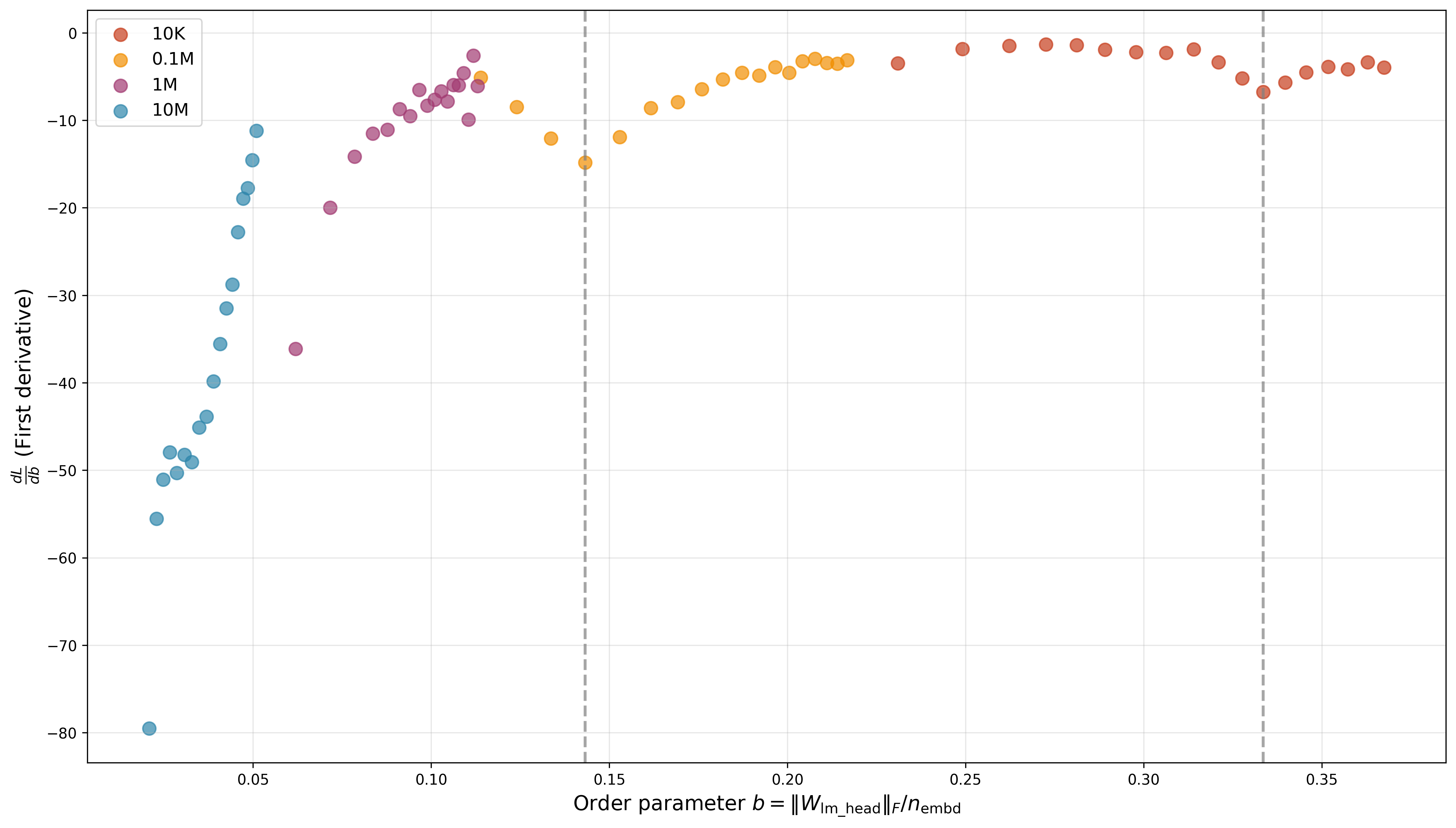
Figure 5: Loss derivative vs LLM Order Parameter shows visible change of slope in case of the smaller 10K and 0.1M parameter models
Conclusion and Next steps
Training a GPT model is easier than you might think. For me, the most satisfying outcome was observing very reasonable performance of a model that can be fully defined and trained using a couple hundred lines of code in ~30mins or so on a local macbook with a GPU.
Statistical physics models, such as the Ising model, have been an inspiration for AI from the very beginning.9 Their principles offer opportunities to probe the dynamics of modern LLMs to improve them and, further, remove their infamous “blackbox” image.
Given additional time and compute resources, I would probably run more experiments to investigate whether this change of slope in the derivative of loss w.r.t to the Ziyin and Ueda8 order parameter actually signifies some kind of phase transition. In the meantime, feel free to play with the code yourself!10
References
-
Radford, A., Narasimhan, K., Salimans, T., & Sutskever, I. (2018). Improving language understanding by generative pre-training. ↩
-
Vaswani, A., Shazeer, N., Parmar, N., Uszkoreit, J., Jones, L., Gomez, A. N., … & Polosukhin, I. (2017). Attention is all you need. Advances in neural information processing systems, 30. ↩
-
Kaplan, J., McCandlish, S., Henighan, T., Brown, T. B., Chess, B., Child, R., … & Amodei, D. (2020). Scaling laws for neural language models. arXiv preprint arXiv:2001.08361. ↩
-
Brush, S. G. (1967). History of the Lenz-Ising model. Reviews of modern physics, 39(4), 883. ↩
-
Ising, E. (1925). Contribution to the theory of ferromagnetism. Z. Phys, 31(1), 253-258. ↩
-
Onsager, L. (1944). Crystal statistics. I. A two-dimensional model with an order-disorder transition. Physical review, 65(3-4), 117. ↩
-
Peierls, R. (1936). On Ising’s model of ferromagnetism. Mathematical Proceedings of the Cambridge Philosophical Society 32(3), 477-481. ↩
-
Ziyin, L., & Ueda, M. (2022). Exact phase transitions in deep learning. arXiv preprint arXiv:2205.12510. ↩ ↩2
-
https://en.wikipedia.org/wiki/Hopfield_network ↩
-
https://github.com/rohitium/LLM-order-param ↩